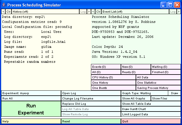
Figure 1: The main simulator window.
The simulator allows you to experiment with various process scheduling algorithms on a collection of processes and to compare such statistics as throughput and waiting time.
Supported algorithms include First-Come/First-Served, Shortest Job First (actually shortest remaining cpu burst time first), and Round Robin. The CPU and I/O bursts of the processes are described by probability distributions, but it is possible to choose the seed so that the same processes can be used to test different algorithms.
The simulator is a Java application that can be run on any platform supporting a modern Java runtime system. The simulator can produce log files in HTML format that include tables of data as well as graphs and Gantt charts.
System requirements:
User requirements:
Running in a non-Windows environment:
If you installed the simulator by copying the files from a CD, the
scripts may not have the correct permissions to run. The convert
and runps files should be executable.
The ASCII files distributed with this distribution are in the Windows format
in which lines end in a carriage return followed by a line feed.
If you are running under UNIX, Linux, or Mac OSX, it
may be more convenient to have the carriage returns removed.
You can remove all of the carriage returns from these files by executing the
convert script.
If you do a custom installation, you can put the jar files anywhere you want. Modify the runps.bat (Windows) or runps (Unix, Linux, Mac OSX) file so that the JARDIR1 or JARDIR2 variable points to the location of the jar files.
If the simulator does not start, make sure you have the Java runtime
executables in your path. In a command window, execute:
java -version
and make sure this displays a version later than 1.0.
An experimental run consists of a scheduling algorithm and a collection of processes to be run under that algorithm. An experiment consists of a number of experimental runs which are to be compared and analyzed. The simulator organizes the input information in order to make it simple to do experiments in which one or more parameters is varied.
To perform an experiment, you must create two files. One file (the run file) contains information about the parameters for the first run. The other file (the experiment file) contains a list of runs to be made and the parameters that vary between runs. The files contain ASCII text so that you can create them directly with a text editor. The standard distribution contains sample files.
After the experiment has been run by the simulator, you can produce tables or graphs of various statistics such as average waiting time and throughput. Information about the experiment including the specification of the processes, the statistics and graphs of the experimental results are stored in a log file in HTML format suitable for viewing from a browser.
The main simulator window is shown in Figure 1.

Figure 1: The main simulator window.
The yellow subwindow in the upper left corner labeled History shows the initial configuration read in from the configuration files. There are three columns of buttons at the bottom of the main window. The leftmost column of buttons allows you to choose the experiment to run and to run it. Pushing the top button in this column advances through the available experiments. Pushing the next button allows you to select which runs of the experiment to do. Pushing the large Run Experiment, runs the chosen experiment.
The second column of buttons controls the log file. The top button allows you to open the log file. When the log file is opened, the button is changed to a Close Log button. As runs are made they are logged in the log file and statistics about the run are saved. Pushing the Log All Table Data button puts two tables of statistics in the log file. The tables contains entries for all selected runs. All runs are selected by default. A sample set of tables is shown in Figure 2.
The first table contains information about average CPU utilization, throughput, turnaround time, and waiting time for each run. The second table contains more detailed information about the turnaround time and waiting time, including the average, the minimum, maximum, and standard deviation for each.
This second column of buttons also has a button for drawing Gantt Charts. See Gantt Charts.
The third column of buttons controls the creation of graphs and tables. At the top are two buttons. The one on the left labeled Graph Type: Waiting will cycle through the types of graphs that can be drawn. Draw the selected type of graph by pushing the Draw button to the right. The entry Graph: Waiting means that a histogram containing information on the waiting time for the processes of each run is to be produced. Each run is displayed in a different color, and the distribution of waiting times is shown as a bar graph. The quantity graphed is the waiting time which is the time spent in the ready queue. Pushing the Draw button pops up a window containing the graph. This window contains a Log button that causes the graph to be inserted in the log file. The sample graph shown in Figure 3 contains waiting time results for an experiment with two runs, one for FCFS and one for SJF.
A more complete explanation can be found in the section Detailed Operation of the Simulator.
| Entries | Average Time | |||||||||
| Description | Algorithm | Time | Processes | Finished | CPU Utilization | Throughput | CPU | I/O | CPU | I/O | myrun_1 | FCFS | 257.05 | 30 | 30 | .96104 | .116711 | 90 | 60 | 2.74 | 15.20 | myrun_2 | SJF | 256.90 | 30 | 30 | .96158 | .116777 | 90 | 60 | 2.74 | 15.20 |
| Turnaround Time | Waiting Time | ||||||||
| Description | Algorithm | Average | Minimum | Maximum | SD | Average | Minimum | Maximum | SD | myrun_1 | FCFS | 215.05 | 169.60 | 257.05 | 31.45 | 176.41 | 138.82 | 202.24 | .66 | myrun_2 | SJF | 124.87 | 62.00 | 256.90 | 62.17 | 86.23 | 16.69 | 229.82 | 2.37 |
Figure 2: Two tables of data created by the simulator when the Log All Table Data button is pushed.
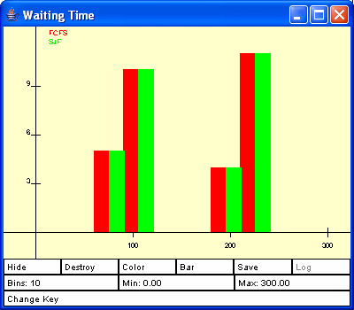
Figure 3: A graph created by the simulator when Graph: Waiting is selected and the Draw Graph button is pushed.
The following distributions are supported:
The file format is as follows:
name experimental_run_name
comment experimental_run_description
algorithm algorithm_description
numprocs number_of_processes
firstarrival first_arrival_time
interarrival interarrival_distribution
duration duration_distribution
cpuburst cpu_burst_distribution
ioburst io_burst_distribution
basepriority base_priority
Here is a sample experimental run file that must be stored in the file myrun.run.
name myrun
comment This is a sample experimental run file
algorithm SJF
numprocs 20
firstarrival 0.0
interarrival constant 0.0
duration uniform 500.0 1000.0
cpuburst constant 50.0
ioburst constant 1.0
basepriority 1.0
This file specifies a run of 20 processes using the shortest job first algorithm. The first process arrives at time 0.0. The interarrival times are all 0.0, so all processes arrive at the same time. Each process has a duration (total CPU time) chosen from a uniform distribution on the interval from 500 to 1000. All processes have a constant cpu burst time of 50 and a small constant I/O burst time of 1.0. The base priority must be present in the file, but it is currently not used by the simulator.
In the simplest case, an experimental run can be specified by the name of the run. In many cases, you will want to make several experimental runs in which almost everything is the same, except that one or more parameters are changed. For example, you might want to vary the quantum used for the round robin scheduling algorithm but use the same set of processes.
The simulator allows you to do this by specifying the same experimental run in each case and giving a new value to one or more parameters. The general format for a run line in the experiment file consists of the word run followed by the name of an experimental run, followed by a list of modifications to that experimental run.
The experiment file format is as follows:
name experiment_name
comment experiment_description
run run_name1 optional_modification_list1
...
run run_namen optional_modification_listn
Here is an example experiment file that must be stored in the file myexp.exp
name myexp
comment This experiment contains 3 runs
run myrun
run myrun cpuburst uniform 10 90
run myrun cpuburst exponential 50
This experiment file makes three runs. All of the runs are based on the run file myrun.run above. In the second run the CPU burst distribution is changed to be uniform in the interval from 10 to 90. In the third run the CPU burst is an exponential distribution with mean 50.
Only the simplest case is described here in which the modification applies to all processes in the run.
A modification specification is a string of tokens separated by one of a small number of key words indicating which parameter is to be modified. The key word may be followed by parameters specific to the value to be modified. For example, if the value to be modified is a distribution, then a distribution is specified in the format described under Probability Distributions. The modification specifications can be in any order.
Here is a list of the key words and the appropriate parameters:
At this time the supported key words are:
logdir .
logfn logfile.html
quiet .
imagename gifim
user Local User
portable true
run myrun
exp myexp
When the log file is opened, the simulator logs information about all of the available experimental runs and experiments. Here is what might be produced for the above configuration.
| Experimental Run Information for 1 Run | |||||||||||||||||||||||||||
| myrun: This contains two types of processes Seed: 0 Algorithm: SJF | ||||||
| Group | Processes | First Arrival | Interarrival | Duration | CPU Burst | I/O Burst |
| 1 | 15 | 0.0 | constant 0.00 | uniform 10.00 15.00 | constant 10.00 | uniform 10.00 20.00 |
| 2 | 15 | 0.0 | constant 0.00 | constant 4.00 | constant 1.00 | uniform 10.00 20.00 |
| Experimental Runs For 1 Experiment | |||
| Experiment | Commentary | Run | Modifications |
| myexp | This experiment contains 2 runs | myrun_1 | algorithm FCFS |
| key FCFS | |||
| myrun_2 | algorithm SJF | ||
| key SJF | |||
Figure 4: The description of an experiment as it might appear in the log file.
The second table describes the experiment that was done which consists of two runs, one using the algorithm FCFS and the other using SJF.
The leftmost text area is labeled History. When active, it displays various information about the progress of the simulation. It also shows the results of any of the information buttons, some of which are located just below the other text area.
The rightmost text area is labeled Event Log. When it is active it shows events are they occur.
Below the Event Log are about a dozen buttons which display information about processes and events of the latest run. There are two types of buttons. The first type appears in a 3 by 3 grid. Each one contains a label with a number if parentheses. When pushed, these buttons immediately display information in the History window. The number in parentheses approximates the number of lines of output generated.
The other buttons are below these in a 2 by 2 grid. These display detailed information about a particular process. When you click one of the other buttons, it will prompt you for a process number. Enter the number and push return to display information about that process. The pointer must be inside the button when data is entered.
Below this is 3 columns of buttons. The first column is for running the simulator. The first button in this column shows which experiment will be run. Pushing this button cycles through the experiments if more than one is listed in the the configuration file. The next button by default is labeled Run All meaning that all runs of this experiment will be done. Pushing this button cycles through the runs for the current experiment, allowing you to execute only that run. The simulator is actually run by pushing the last of these buttons, labeled Run Experiment.
The second column is mainly for logging the results of the simulator. The last column if for displaying various tables and graphs. These are described below.
The second column of buttons is primarily related to logging of data.
The third column of buttons is primarily related to tables and graphs. Figure 2 show a window that appears when you push the Drawh button. Graphs can be resized and you can modify various parameters used to draw the graph. You can set the number of bins as well as the minimum and maximum value graphed. To change these, click the mouse in the appropriate button and you will be prompted for the new value. If setting the minimum or maximum causes some processes to not be displayed, the number of missing processes is displayed in the min and max box in parentheses.
The Change Key button can be used to change the key in the graph. If there is more than one run displayed, pushing this button prompts for the index of the run to change. The index numbers appear with the keys on the graph when this occurs. After choosing a run, enter the new key. In a similar way, the Color button allows you to change the color used to graph a particular run. After choosing the index, click on the color you want to use.
Below the buttons are two narrow progress bars showing the progress of the simulation. The first is red and shows the fraction of total CPU time that has been used so far. When the red bar reaches the end, all processes are complete. The second progress bar is blue and shows the fraction of processes that have completed.
Finally, at the bottom of the window are three buttons.
There are times when you may want to repeat an experiment or run in order to look at it in more detail. The option portable true allows you to do this. The simulator uses a portable pseudo-random number generator with a fixed seed so that if the same run is repeated, it should produce exactly the same results. The seed is reset at the start of each run, so that a run is not affected by previous runs.
By default, the simulator uses one random number generator for calculating all distributions. CPU bursts and I/O bursts for processes are calculated on the fly for each process when they are needed. A CPU burst times is calculated when the process enters the ready queue. Since the scheduling algorithm can affect the order in which processes enter the ready queue, the same set of processes running under different scheduling algorithms will have different burst times. This makes it difficult to compare the algorithms.
If a seed value is specified in the Experimental Run file, independent random number generators are used for each instance of a distribution. This implies that if the same creator is used to create processes which are run through different algorithms, those processes will have exactly the same values for the CPU and I/O bursts for both runs.
Pushing this button brings up a window containing one line for each run that has been finished. Each line contains the name of a run and two buttons. Pushing the Log button changes it to NoLog and indicates that the corresponding run should not be included. Pushing the same button again resets it. The other button is marked Show. When it is pushed the line disappears from the data editor window. You can show the missing lines by pushing the Show Some button which changes it to Show All. Pushing it again resets it. When finished, you can push the Done button.
The first optional line contains one of three words, priorityoff, priorityon, or prioritypreempt corresponding to no priority, non-preemptive priority, and preemptive priority, respectively.
The second optional line starts with the key word key followed by a parameter which is the key to be used in the waiting time graphs. It could be any string.
The third optional line starts with the key word seed and has a parameter which is an integer. This is used to initialize the random number generator. See Random and Not So Random Numbers.
The fourth and fifth optional lines specifiy the context switch time. See Context Switch.
The file contains any number of sets of 7 lines giving the number of processes, first arrival time, interarrival distribution, duration distribution, cpu burst distribution, io burst distribution and base priority as discussed earlier.
The file format is as follows with at most one of the blue lines and either or both of the red lines and the block of seven magenta lines repeated any number of times.
name experimental_run_name
comment experimental_run_description
algorithm algorithm_description
priorityoff
priorityon
prioritypreempt
key key_string
seed seed_value
cstin context_switch_time_in
cstout context_switch_time_out
numprocs number_of_processes
firstarrival first_arrival_time
interarrival interarrival_distribution
duration duration_distribution
cpuburst cpu_burst_distribution
ioburst io_burst_distribution
basepriority base_priority
Here is a sample run file which uses the second format which would be stored in the file thisrun.run:
name thisrun
comment This specifies two types of processes
algorithm FCFS
priorityon
key Non-preemptive FCFS with processes having two priorities
numprocs 10
firstarrival 0.0
interarrival constant 1.0
duration uniform 500.0 1000.0
cpuburst constant 50.0
ioburst constant 1.0
basepriority 1.0
numprocs 30
firstarrival 0.0
interarrival constant 1.0
duration uniform 50.0 100.0
cpuburst exponential 20
ioburst exponential 500
basepriority 2.0
This defines two types of processes, 10 of which are longer running use little I/O, and are of low priority and 30 of which are relatively short, use more I/O and have higher priority. The scheduling algorithm is non-preemptive First-Come, First-Served using fixed process priorities.
During a context switch in, the process remains int he ready queue so this time contributes to the waiting time of the process. When a context switch out occurs, the process changes state immediately to a switching state. In the Gantt charts, this is shown as a block space. If I/O is requested the I/O is delayed until the context switch out is done. If the process was preempted, it does not arrive in the ready queue until the context switch out is done.
  Runs read:         5 of 5
  Experiments read:  3 of 3
The Draw Gantt Chart button in the last column of buttons is for producing Gantt Charts. If more than one run has been made, a menu pops up allowing you to choose which run to use. Select one of the runs and a Gantt Chart will be displayed. If only one run has been done, this step is skipped. A sample Gantt Chart is shown in Figure 5.
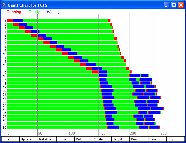
Figure 5: A Gantt Chart.
The Log button can be used to put a copy of the Gantt chart in the log file. This might take a while on a slow machine as each pixel needs to be grabbed from the image and then converted to a GIF file. The Controls displays additional sliders for controlling the height and spacing of the bars. It is possible to get a useful Gantt Chart of hundreds of processes by making the bars 1 pixel high. Figure 6 shows the controls window. Figure 7 shows two Gantt chars, each with 200 processes, one for FCFS and one for SJF. Figure 8 shows a zoomed in view of one of these.
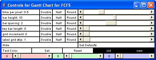
Figure 6: Gantt Chart Controls.
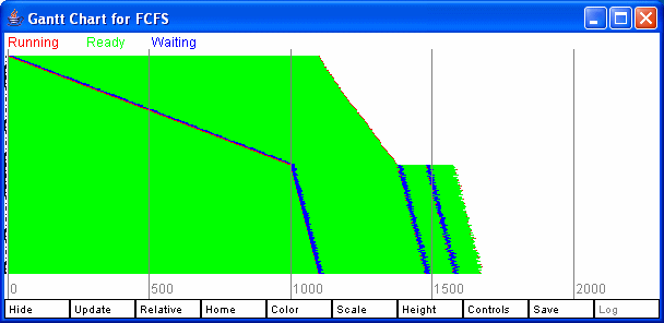
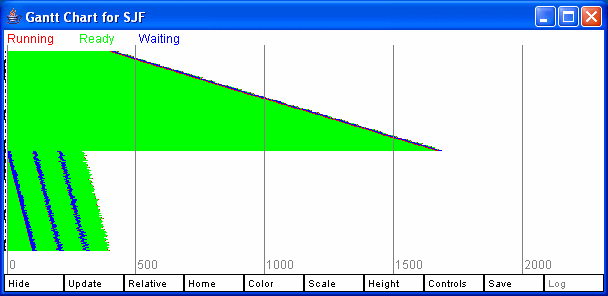
Figure 7: Two Gantt Charts, each with 200 processes.
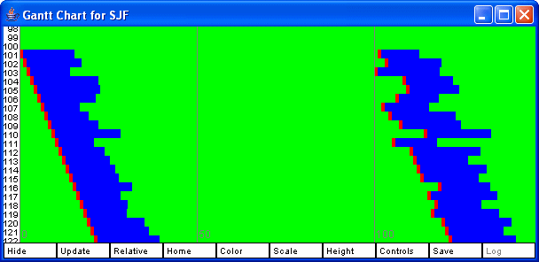
Figure 8: A zoomed in view of a Gantt Chart from Figure 7.
Each of these windows has a Clr button at the top to empty it of text and a Log button which is active whenever the log is open. Pushing this button inserts a copy of the contents of the box into the log file.
There are two small buttons on either end of the top of these boxes. Pushing the leftmost one reduces the size of the font displayed while pushing the rightmost one increases the size of the font. These do not affect what gets put into the log file.
I/O bursts of 0 are treated as very small I/O bursts. This means that when a process finishes its CPU burst the scheduler picks a different process from the ready queue and then puts the process back in the ready queue. Only if the ready queue was empty will that same process be given the CPU again.