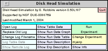
Figure 1: The main simulator window.
Before starting the simulator, edit the file diskheadconfig and change the user line to contain your name instead of New User. Start the simulator by executing rundisk.
If all goes well the simulator will start up and look something like Figure 1.
Figure 1: The main simulator window.
The figure shows a small window with a number of colored buttons in three columns.
Push the green Run Experiment button on the right side of the window. The Run Experiment button will briefly change color and become a Pause Experiment before returning to its original form. When it does, the experiment has completed.
The experiment consists of running the simulator three times with different seek movement algorithms, FCFS, SSTF and C-LOOK. Push the Show Table Data button which is located at the top of the second column of buttons. You should see a window showing statistics of the run similar to the one shown in Figure 2.
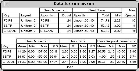
Figure 2: Statistics generated by the simulator.
Two tables are shown. The upper table shows the algorithm name and the number of seeks under the heading Seek Movement. Under Seek Time three items are shown. The first is the algorithm for calculating how long it takes to move from one cylinder to another. Linear 0.5 .10 means it takes .5 ms plus .10 ms per cylinder. The next value is the time the last seek completed and this is followed by the idle time, the total time that no seeks are taking place. The last column gives the maximum number of pending seek requests.
The lower table gives detailed statistics for each of the runs, giving the mean, minimum, maximum and sample standard deviation for three different statistical measures. Seek Movement refers to the number of cylinders moved. Seek Time is the time it takes to perform a seek using the seek time algorithm listed in the table above. The Seek Request Turnaround refers to the time between when a request comes in and the time the corresponding seek has completed.
Close the table data window by pushing the Done button at the bottom of the window. Find the Show Run Data Graph button and click on it. This should popup a small window. Choose all runs and three diagrams will appear, one for each run. The head position is shown on the horizontal axis. The vertical axis corresponds to changes in the direction of head movement.
Find the Show Run Data Table button and click on it. Choose the SSTF entry. This will display a table similar to Figure 3, showing each individual seek in the order that the seek is started. For each seek, the starting and ending block number are shown. This is followed by the time the seek request arrived, the time is started and the time it completed. The turnaround time is shown next. This is the time between the request and the completion of the seek. Lastly, the size of the queue of pending requests at the time the request arrived is shown.
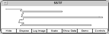
Figure 3: Seek data for SSTF.
The Seek Time or movement algorithm determines the time it takes
to move from one cylinder to another. The simplest of these is the linear algorithm
in which the time is a linear function of the number of cylinders to move. It is
specified by two parameters. If you think of the time as the y-axis and the
number of cylinders to move on the x-axis, the two parameters are the y-intercept and
the slope. In Figure 2, the movement algorithm is shown in the Algorithm column
under Seek Time. In this experiment all runs use the same algorithm:
Linear .50 .10 which
would be specified in the configuration file as:
movement linear 0.5 0.10
This means that it the time it takes to do a seek is 0.5 ms plus 0.1 ms per cylinder.
This algorithm is only used when seeking a new cylinder.
A seek that does not change cylinders does not take any time.
The Layout algorithm indicates how sectors are laid out on the disk. The
simplest layout algorithm uses a constant number of sectors per track and is called
Uniform. The simulator does its scheduling in terms of blocks which
are the same as sectors, but the
blocks consecutively numbered starting at 0. It uses the
layout algorithm to determine which cylinder a given block is on. The layout
algorithm is shown in Figure 2 in the Layout column. The specification
Uniform 2 means 2 blocks per cylinder.
For a uniform layout with n blocks per cylinder, the cylinder number is obtained by
dividing the block number by n and truncating the result.
The uniform layout with 2 blocks per cylinder would be
specified in the configuration file as:
layout uniform 2
In Figure 3, the first line of the table show a seek from block 4 to block 36. With a uniform 2 layout, block 4 is on cylinder 2 and block 36 is on cylinder 18. The head has to move 16 cylinders. This takes 0.5 + 16*(0.1) = 2.1 ms. This number is shown in the Seek Time column of Figure 3.
Each run line starts with the key word run followed by a name which
specifies a file with extension .run. For example, the run line:
run myrun
specifies a file called myrun.run
A run file specifies everything about a run, including the three types of algorithms described above as well as the starting block number and the seek requests. Seek requests can be specified in two ways, either by giving an explicit sequence of requests or by generating requests with probability distributions.
A line in the run file of the form
input abc
specifies a file called abc that contains a sequence of block requests.
Each line of the file should contain two tokens, a time at which the request is made
a floating point number) and a block number (an integer).
Alternatively, requests can be specified with probability distributions. A set of
requests is specified by giving the first arrival time, an interarrival time
distribution, and a distribution for block requests. For example, the lines:
interArrival constant 2
nextBlock uniform 30 40
firstArrival 2.23
numBlocks 20
indicate that 20 blocks are described, the first arriving at time 2.23.
After that the interarrival time is a constant 2 ms and requested block is
chosen uniformly from between 30 and 40. The 4 lines specifying a distribution
of block requests can occur in any order, but all 4 must be given before another
set of block requests can be specified.
An experiment consists of a number of runs with almost identical parameters.
An experiment is described in a file with extension .exp. After the initial
two lines of the file containing the name and a comment, each line specifies a run to
be made. A run line in an exp file starts with the key word run followed
by the name of a run file (without the .run extension). This may optionally be
followed by a number of run modifiers. Each run modifier changes a parameter of the
run. For example, the following is the experiment file for the examples in the
figures above:
name myexp
comment This is a test
run myrun key "FCFS" head FCFS
run myrun key "SSTF" head SSTF
run myrun key "C-LOOK" head CLOOK
This specifies three runs all using the same run file. The runs differ only the
head algorithm, that is the algorithm used to determine the next request to
satisfy given a list of pending requests. Also modified is the key, a string
that is used to identify the run. The key for each run is shown in the first column
in Figure 2.
Other run modifiers can change the layout or movement algorithm.
While running the simulator, you can push the Show Run Description button to show a description of all of the runs of the current experiment. The Show Exp Descrition button shows the contents of the exp file for the current experiment.
When the log file is open, it will include information about each run made. The Log Table Data will include a table of statistics in the log file similar to the one shown with the Show Table Data button. Most of the other windows that the simulator displays have log button that is active when the log file is open. This inserts the corresponding infomation in the log file.
Start the simulator and click on the Open Log button.
Push the Run Experiment button and then try each of the following
buttons:
Show Run Data Graph followed by all runs
Show Run Data Table followed by FCFS
Show Run Description
Show Exp Description
Include these in the log file.
Close the log file and then look at the log file in a browser.