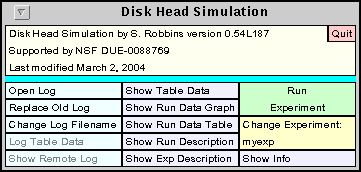
Figure 1: The main simulator window.
The time to do a seek can be set to be any linear function of the number of cylinders to move. The simulator supports both a uniform layout of blocks (a fixed number of blocks per cylinder) or a zoned layout in which the physical disk is divided into sections with different uniform layouts.
The simulator assumes that the operating system is doing the scheduling. It can either assume that the operating system has complete knowledge of the physical layout of the disk or the operating system can use a different layout. For example, the operating systems can use LBA (logical block addressing) in which it essentially assumes that each block is on a separate cylinder while the physical layout is zoned. The consequences of this mismatch can be explored using the simulator.
The simulator can generate graphs and tables of statistics which can be used to compare different disk layouts or seek algorithms. All data and graphs generated by the simulator can be placed in a log file in HTML format for display or printing.
The simulator is available for download and is freely available.
System requirements:
User requirements:
Running in a non-Windows environment:
If you installed the simulator by copying the files from a CD, the
scripts may not have the correct permissions to run. The convert
and rundisk files should be executable.
The ASCII files distributed with this distribution are in the Windows format
in which lines end in a carriage return followed by a line feed.
It may be more convenient to have the carriage returns removed.
If you are running under UNIX, Linux, or Mac OSX, it
may be more convenient to have the carriage returns removed.
You can remove all of the carriage returns from these files by executing the
convert script.
If you do a custom installation, you can put the jar files anywhere you want. Modify the rundisk.bat (Windows) or rundisk (Unix, Linux, Mac OSX) file so that the JARDIR1 or JARDIR2 variables points to the location of the jar files.
If the simulator does not start, make sure you have the Java runtime
executables in your path. In a command window, execute:
java -version
and make sure this displays a version later than 1.0.

Figure 1: The main simulator window.
After running the experiment, the results can be displayed using the Show Table Data at the top of the middle column. This displays information about the result of the runs. Figure 2 shows the table for three runs.
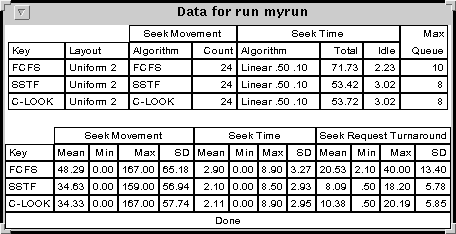
Figure 2: The statistics generated by the simulator.
The Show Run Data Graph displays a graphical representation of one of the runs. If more than one run has been made, you will be presented with a list of runs to choose from. After choosing one of these, a graph of the selected run will appear. Figure 3 below shows a graph for the SSTF algorithm applied to the following track numbers:

Figure 3: A graphical representation of the SSTF algorithm.
The data and graphics generated by the simulator can be saved in an HTML file that can be displayed and printed by a standard browser. See the section on logging.
| Keyword | Values | Meaning |
| user | anything | The name of the current user. This appears in the log file. |
| quiet | none | Turns off all sounds generated by the simulator. |
| run | a filename | This is the name of a file with extension .run. The extension is not listed. Each run file used by the simulator must have a corresponding run line in the configuration file. |
| exp | a filename | This is the name of a file with extension .exp. The extension is not listed. Each exp file used by the simulator must have a corresponding run line in the configuration file. |
| input | a filename | The name of an input file. Each input file specified in a run or exp file must appear here. |
| fontsize | an integer | The default fontsize. This parameter is optional. |
| fontname | a font name | This must be the name of a font that is recognized by the Java system. It is optional. |
| fontstyle | a font style | This is either plain, bold or italics. It is optional. |
| logdir | a directory path | If given, this is the directory for storing the log file. If not given, the log file is stored in the current directory. |
| logfile | a filename | The name of the log file. The extension .html will be appended to this. The default log file is logfile.html. |
| imagename | a filename | This is the base filename used for images created for the log file. The default is gifimage. |
| datadir | a directory path | If given, this is where input, run and exp file are located. By default, they are stored in the current directory. |
| port | an integer | If this value is greater than zero, remote logging will be used with this port. The default is 0. |
| standardcolors | 4 integers | If given, these numbers affect the intensity of the colors used by the simulator. |
The following lines of the run file contain the following information:
| Keyword | Values |
| key | Text describing the run. This is used in many of the tables to distinguish this run from others. |
| doublebuffer | Either true or false. If true, new requests are put in a separator pending buffer until previous requests have been handled. When the current buffer is empty, the pending buffer becomes the current one. The default value is false. |
| input | A file name. The file contains a list of blocks to seek along with arrival time. Each line of the file contains an integer block number and a floating point arrival time. Multiple input lines can be used and the associated files are merged. Input files can also be combined with seek blocks generated by distributions as described below. |
| seed | An integer used to seed the random number generator used for the simulations. If specified it allows repeated simulations to generate identical results. |
| seedtime | Either true or false. If true, the seed is generated from the current time (with millisecond precision) and any seed specified with the seed keyword is ignored. The default is false. |
| start | An integer representing a block number. This is the starting block number of the disk head. The default is 0. |
| layout | The value has one of two forms: ����� uniform n, where n is an integer ����� zoned n1 m1 n2 m2 ... The first form is for a uniform layout with n blocks per cylinder. The second form is for a zoned layout in which ni is the number of blocks per sector and mi is the number of sectors in the ith zone. This represents the physical layout of the disk, used to determining how long it takes to perform a seek. Each run file must have exactly one layout entry. |
| oslayout | The value parameter is the same as for the layout keyword. If specified, this is the layout assumed by the operating system. It is used to determine which block to seek next and where the operating system thinks the disk head is currently positioned. It defaults to the physical layout. |
| movement | This specifies how long it takes the disk head
to move from one cylinder to another. The only currently supported
movement algorithm is linear and specified by ����� linear n m where n and m are integers. The time for a seek of x cylinders for x greater than 0 is nx + m. A seek of zero always takes 0 time. Each run file must have exactly one movement entry. |
| badfraction | The value is a floating point number between 0 and 1. It represents the fraction of references that are to bad blocks. A reference to a bad block is mapped to a location given by the baddestination keyword. It value defaults to 0. |
| baddestination | The value parameter is a distribution. See the section on Probability Distributions for the format. This entry is necessary when badfraction is not 0. When a bad block is referenced, this distribution is used to generate the actual destination. |
| head | The value is one of the following specifications
that determine when block to seek next. ����� FCFS ����� SSTF ����� LOOK ����� LOOK- ����� CLOOK ����� SCAN n ����� SCAN- n ����� CSCAN n ����� V x y ����� V- x y These are described in more detail under Head Algorithms. |
| clear | This keyword does not use a value. The clear keyword is used in run modifications (described below) to remove any block requests specified in a run file |
| numblocks | The value is an integer specifying the number of block requests to generate from a distribution. The four keywords numblocks, firstarrival, interarrival and nextblock form a set and must all be present to specify a set of blocks to generate. The blockabsolute and blockrelative are optional keywords that modify the set of blocks. Multiple sets many be specified. |
| firstarrival | The value is a floating point number representing the arrival time of the first block generated in this set. |
| interarrival | The value is a distribution specification giving the interarrival time of the requested blocks. |
| nextblock | The value is a distribution specification that is used for generating the next block request. |
| blockabsolute | This does not take any parameters. This is the default which indicates that the distribution given by the nextblock keyword generates absolute block numbers. |
| blockrelative | This does not take any parameters. If given, it specifies that the block numbers generated by the nextblock distribution are relative to the previous block generated. This feature is not implemented in the current version of the simulator. |
An experiment performs several runs and compares the results. An experiment is described by a file with extension .exp. Like the run file, it consists of lines containing keywords and values. The first two lines of an experiment file contain a name and comment field similar to those of a run file. The name line contains the name of the file without the .exp extension. The rest of the lines in an experiment file contain the keyword run followed by the name of a run file.
The name of the run file may be followed by any number of keyword-value pairs that modify the run. The keywords and values are the same as those listed in the table. The run modifications allow the same run file to be used several times in the same experiment.
For example, suppose that the file myrun.run uses the FCFS head movement algorithm. The following file called myexp.exp will make three runs, all with the same parameters but using three different head movement algorithms:
name myexp
comment Three head algorithms compared
run myrun key "FCFS"
run myrun key "SSTF" head SSTF
run myrun key "C-LOOK" head CLOOK
The first run line has one modification, key while the others modify both the key and the head. Any modifications in the run line of an experiment file override the corresponding value in the named run file.
The following distributions are supported:
| Algorithm | Argument types | Description |
| SCAN | integer | The SCAN algorithm starts moving the head toward higher cylinder numbers until it reaches the last cylinder (given by the argument) stopping at pending blocks along the way. It then reverses direction and stops at pending blocks on the way back, moving al the way to cylinder 0. |
| SCAN- | integer | This is similar to the SCAN algorithm, but it starts moving toward lower cylinder numbers. |
| CSCAN | integer | This is similar to SCAN but does not stop at pending blocks on the way bak to cylinder 0. |
| LOOK | none | LOOK is like SCAN, but it changes direction when there are no more pending blocks in the current direction. |
| LOOK- | none | This is like LOOK but it starts moving towards lower block numbers. |
| CLOOK | none | This is like CSCAN but it changes directions when there are no more pending references. |
| FCFS | none | This seeks blocks in the order in which they are requested. |
| SSTF | none | The next block to seek is on the cylinder closest to the current one. |
| V | float integer | This is the Vr algorithm that takes two parameters, x and y. x is a floating point value between 0 and 1. and y is an integer representing the largest block number. This algorithm is a mixture of SSTF and SCAN with the x parameter indicating the mix. When x = 0 the algorithm is SSTF and when x = 1 the algorithm is SCAN. |
| V- | float integer | This is like V but starts in the direction toward lower block numbers. |
In addition, double buffering may be specified for each algorithm.
In a zoned layout, the disk is divided into zones, each one having a uniform
layout. A zoned layout is specified by giving the number of zones, n
followed by n pairs of integers, each giving the number of cylinders
in that zone and the number of blocks per cylinder for that zone. For example,
layout zoned 3 10 8 10 16 10 24
would represent a disk with 3 zones, of 10 cylinders each. The first 10
cylinders have 8 blocks per cylinder, the next 10 have 16 blocks per
cylinder and the last 10 have 24 blocks per cylinder.
The simulator allows for two different layouts, one the physical layout
of the disk and the other being the logical view of the disk by the
operating system. By default these are the same, but the layout as seen by the
operating system may be set independently with the oslayout
keyword. For example
layout zoned 3 10 8 10 16 10 24
oslayout uniform 16
indicates that the physical disk is zoned as above, but the operating system
thinks that it is uniform.
The operating systems layout is used to determine the next block to seek while the physical layout is used (along with the movement algorithm) to determine how long it takes to perform the seek.
The head algorithm is used to decide which block to seek next from a list of pending block requests. The simulator uses two methods for generating these block requests. For a short list of requests, the simplest methods is to just specify each requested block number along with the time at which the request is made. Use the input keyword with the name of a file as its one value to specify a file containing such a list. The format of this file is a sequence of lines, each containing a time (floating point value) followed by a block number (an integer). The lines of this file do not have to be in any particular order. More than one input file may be specified and you can specify both input files along with distributions described below.
An alternative to presenting a list of block numbers is to have the simulator generate block numbers using distributions. A collection of block numbers is specified with distributions by specifying four keyword-value pairs:
| Keyword | Value |
| numblocks | An integer specifying how many block requests will be generated. |
| firstarrival | A floating point value indicating the time at which the first of these blocks arrives. |
| interarrival | A distribution giving the interarrival times of the generated blocks. |
| nextblock | A distribution used to generate the block request. |
The four keyword-value pairs may occur in any order. Multiple distributions of block requests can be used by repeating these four keyword-value pairs.
If used in a run modification, the input file or distribution specifications add additional block requests to those specified in the run file. To clear all block request specifications, use the keyword clear.

Figure 1 (repeated): The main simulator window.
The large yellow button in the third column shows the name of the current experiment. If more than one experiment was specified in the configuration file, pushing this button changes to another experiment. Pushing the large green Run Experiment runs the current experiment. Pushing this button splits it into two buttons: Pause Experiment and Abort Experiment until the experiment is complete. When the experiment has completed, the button changes back to its original form. If the Pause Experiment button is pushed while the experiment is running, the experiment is temporarily stopped and this button changes into a Continue Experiment button. Pushing this button resumes the experiment. Pushing the Abort Experiment button ends the experiment and no data from the experiment is saved.
The remaining 6 buttons display information about completed runs.
The Show Table Data Button show a table of statistics for all of the runs similar to the one in the figure below.

Figure 2 (repeated): The statistics generated by the simulator.
Each run is labeled by its key. The top part of the table shows the three algorithms used by this run, the layout algorithm, the seek movement (or head) algorithm and the seek time (or seek movement) algorithm. Also shown are the number of seeks (Count column), the total and time seeking, the total idle time (when no head movement is occurring) and the maximum queue length.
The bottom part of the table gives detailed numeric data about the seek movement (number of tracks moved per seek), the seek time, and the seek request turnaround time. This latter time is the time between when the seek request is make and when the seek is completed. For each of these four statistics, the main, minimum, maximum and sample standard deviation are given.
The Done button at the bottom of the window is used to close the window.
The Show Run Data Graph allows you to select a run. When selected, a graphic showing the head movement is displayed. The figure below shows the Shortest Seek Time First (SSTF) graphic corresponding to the run in above table.

Figure 3 (repeated): A graphical representation of the SSTF algorithm.
The horizontal direction corresponds to head position. Each time the head changes direction, the trace moves down. A tic mark appears each time a seek position is reached that does not cause a change in direction. The buttons on the bottom of the provide some additional features. The Hide button temporarily hides the window. It can be brought back again using the Show Run Data Graph button. The Dispose button permanently destroys the window and all its resources. If the Show Run Data Graph button is used again for this run, a new window is created. If logging is active, the Log button will put a copy of this image (without the buttons) in the log file. The Scale button will attempt to rescale the graphics so that it entirely fits in the window. The Show Data button pops up the same table available through the Show Run Data Table of the main simulator window. It will be described later. The Demo button enters Demo Mode for this window. This mode is described in the section on Demo Mode. Lastly, the Controls window allows you to set the scale and colors of various features of this window.
The Show Run Data Table button shows a detailed table of data about all of the seeks made in the given run. The figure below shows the table for the SSTF run corresponding to the above graphic.
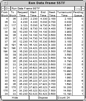
Figure 4: The table generated by the Show Run Data Table button.
For each seek it shows the starting and ending block, the time the request was made, the time the seek started, the time the seek ended, the time to do the seek (the difference of the previous two entries), the turnaround time (between request and completion) and the size of the pending queue when the request was made. At the bottom of the table, the total number of seeks for this run is shown. Two button at the bottom of the table allow you to hide or dispose of the window.
The Show Run Description button gives a description of the runs from the current experiments. This is essentially the contents of the run file modified by the modifications in the exp file. The table for the experiment shown in Figure x is given in the table below.
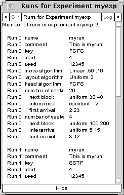
Figure 5: The table generated by the Show Run Description button.
The Show Exp Description button shows the contents of the exp file for the current experiment. The figure below shows an example.
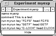
Figure 6: The table generated by the Show Exp Description button.
The Show Info button displays a window giving a log of the runs made. It logs events (with wall clock time) such as the start and completion of each run. The window generated for the above run is shown below. The Scale button attempts to fit all of the data in the window if there are more lines than are currently displayed. Otherwise there will be a scroll bar on the right side of the window.
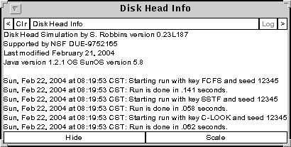
Figure 7: The table generated by the Show Info button.
The tables of data shown in Figures x, y, z, ... have a common format. They can all be resized. If the data to be displayed does not fit in the current format, scroll bars appear on the bottom or right side of the window. At the top of each window are two small buttons on either side. The <: and >l buttons will respectively decrease or increase the size of the font. If the Clr button is active it will clear the contents of the window. If logging is active, the Log will put a copy of the table in the log file.
The name and location of the log file is controlled by logfile and logdir configuration parameters. The simulator will store images in the logging directory with a name based on the imagename configuration parameter.
You can change the name of the log and image files after the simulator starts by using the Change Log Filename button. This will allow you to change the logging directory, the filename and the image filename.
Normally, when you open a new log file it will replace an existing log file of the same name. Pushing the Replace Old Log button changes it to Append To Old Log and causes future opens to append to and existing log file of the same name. It also modifies the image file name so that images created do not interfere with those created previously.
Open the log file by pushing the Open Log button. This changes the Open Log button to Close Log so that the log can be closed. It also changes the the buttons to Log Comment and Stop Log. The Log Table Data is activated.
The Log Comment button allows you to insert a comment into the log file. The Stop Log button changes to Start Log when pushed and allows you to temporarily stop and restart automatic logging without closing the log file.
The Log Table Data button inserts a table of data into the log file. The information in this table is similar to the information displayed with the Show Table Data button.
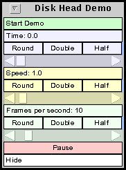
Figure 8: The control panel for demo mode.
This control panel allows you to control the simulator time. It contains a Start Button, a Time Slider, a Speed Slider, an Update Rate slider, and Pause/Resume button and a Hide button. Each of the sliders controls a particular quantity and consists of three rows of widgets of the same color. The first widget shows the value of the quantity being controlled. The second row contains three buttons. The first button rounds the value. The Double and Half buttons control the upper limit of the slider value. The third row contains the slider.
You can either set it manually by moving the time slider or to automatically run the time at a fixed rate by pushing the Start Demo button. The speed at which time progresses is controlled the Speed Slider. How often the graphs update is controlled by the last slider, labeled Frames per second. Next there is the Pause button. When it is pushed, the simulation time stops and the button changes to a Resume button. Lastly, the Hide button hides the demo control window. You can bring this window back by turning off and on the demo in any of the run data graph displays.
 |
 |
 |
Figure 9: Demo mode.
Figure 9 shows graph displays of three algorithms in demo mode along with the demo control panel. The time is paused at 44.695. Each of the graphs shows the state of the simulation at that time. At the top of each graph are tick marks in blank, green and red. The black marks are pending requests. The request of the current seek is shown in green. The current head position is shown in red.